Query nodes with spatial predicates

These functions allow to interpret spatial relations between nodes and other geospatial features directly inside filter and mutate calls. All functions return a logical vector of the same length as the number of nodes in the network. Element i in that vector is TRUE whenever any(predicate(x[i], y[j])) is TRUE. Hence, in the case of using node_intersects, element i in the returned vector is TRUE when node i intersects with any of the features given in y.

node_intersects(y, ...)

node_is_disjoint(y, ...)

node_touches(y, ...)

node_is_within(y, ...)

node_equals(y, ...)

node_is_covered_by(y, ...)

node_is_within_distance(y, ...)

Arguments

y

The geospatial features to test the nodes against, either as an object of class sf or sfc.

...

Arguments passed on to the corresponding spatial predicate function of sf. See geos_binary_pred.

Value

A logical vector of the same length as the number of nodes in the network.

Details

See geos_binary_pred for details on each spatial predicate. Just as with all query functions in tidygraph, these functions are meant to be called inside tidygraph verbs such as mutate or filter, where the network that is currently being worked on is known and thus not needed as an argument to the function. If you want to use an algorithm outside of the tidygraph framework you can use with_graph to set the context temporarily while the algorithm is being evaluated.

Note

Note that node_is_within_distance is a wrapper around the st_is_within_distance predicate from sf. Hence, it is based on 'as-the-crow-flies' distance, and not on distances over the network. For distances over the network, use node_distance_to with edge lengths as weights argument.

Examples

library(sf, quietly = TRUE)
library(tidygraph, quietly = TRUE)

# Create a network.
net = as_sfnetwork(roxel) %>%
  st_transform(3035)

# Create a geometry to test against.
p1 = st_point(c(4151358, 3208045))
p2 = st_point(c(4151340, 3207520))
p3 = st_point(c(4151756, 3207506))
p4 = st_point(c(4151774, 3208031))

poly = st_multipoint(c(p1, p2, p3, p4)) %>%
  st_cast('POLYGON') %>%
  st_sfc(crs = 3035)

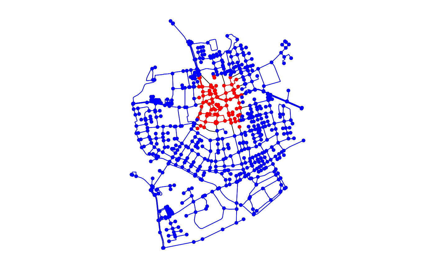
# Use predicate query function in a filter call.
within = net %>%
  activate("nodes") %>%
  filter(node_is_within(poly))

disjoint = net %>%
  activate("nodes") %>%
  filter(node_is_disjoint(poly))
oldpar = par(no.readonly = TRUE)
par(mar = c(1,1,1,1))
plot(net)
plot(within, col = "red", add = TRUE)
plot(disjoint, col = "blue", add = TRUE)

par(oldpar)

# Use predicate query function in a mutate call.
net %>%
  activate("nodes") %>%
  mutate(within = node_is_within(poly)) %>%
  select(within)
#> # A sfnetwork with 701 nodes and 851 edges
#> #
#> # CRS:  EPSG:3035 
#> #
#> # A directed multigraph with 14 components with spatially explicit edges
#> #
#> # A tibble: 701 × 2
#>   within          geometry
#>   <lgl>        <POINT [m]>
#> 1 TRUE   (4151491 3207923)
#> 2 TRUE   (4151474 3207946)
#> 3 TRUE   (4151398 3207777)
#> 4 TRUE   (4151370 3207673)
#> 5 TRUE   (4151408 3207539)
#> 6 TRUE   (4151421 3207592)
#> # ℹ 695 more rows
#> #
#> # A tibble: 851 × 5
#>    from    to name                  type                                geometry
#>   <int> <int> <chr>                 <fct>                       <LINESTRING [m]>
#> 1     1     2 Havixbecker Strasse   residential (4151491 3207923, 4151474 32079…
#> 2     3     4 Pienersallee          secondary   (4151398 3207777, 4151390 32077…
#> 3     5     6 Schulte-Bernd-Strasse residential (4151408 3207539, 4151417 32075…
#> # ℹ 848 more rows