3. Spatial joins and filters
2026-05-14
Source:vignettes/sfn03_join_filter.Rmd
sfn03_join_filter.RmdThe integration with sf and addition of several spatial
network specific functions in sfnetworks allow to easily
filter information from a network based on spatial relationships, and to
join new information into a network based on spatial relationships. This
vignette presents several ways to do that.
Both spatial filters and spatial joins use spatial predicate
functions to examine spatial relationships. Spatial predicates are
mathematically defined binary spatial relations between two simple
feature geometries. Often used examples include the predicate
equals (geometry x is equal to geometry y) and the predicate
intersects (geometry x has at least one point in common with
geometry y). For an overview of all available spatial predicate
functions in sf and links to detailed explanations of the
underlying algorithms, see here.
Spatial filters
Using st_filter
Information can be filtered from a network by using spatial predicate
functions inside the sf function sf::st_filter(), which
works as follows: the function is applied to a set of geometries A with
respect to another set of geometries B, and removes features from A
based on their spatial relation with the features in B. A practical
example: when using the predicate intersects, all geometries in
A that do not intersect with any geometry in B are removed.
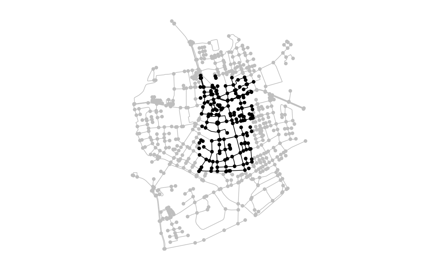
When applying sf::st_filter() to a sfnetwork, it is
internally applied to the active element of that network. For example:
filtering information from a network A with activated nodes, using a set
of polygons B and the predicate intersects, will remove those
nodes that do not intersect with any of the polygons in B from the
network. When edges are active, it will remove the edges that do not
intersect with any of the polygons in B from the network.
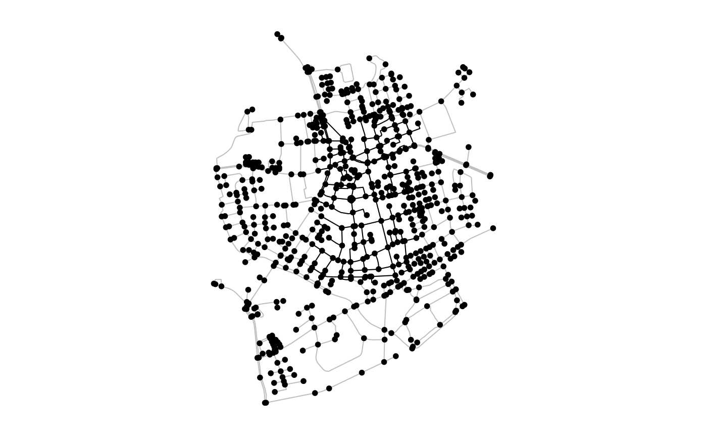
Although the filter is applied only to the active element of the
network, it may also affect the other element. When nodes are removed,
their incident edges are removed as well. However, when edges are
removed, the nodes at their endpoints remain, even if they don’t have
any other incident edges. This behavior is inherited from
tidygraph and understandable from a graph theory point of
view: by definition nodes can exist peacefully in isolation, while edges
can never exist without nodes at their endpoints.
p1 = st_point(c(4151358, 3208045))
p2 = st_point(c(4151340, 3207120))
p3 = st_point(c(4151856, 3207106))
p4 = st_point(c(4151874, 3208031))

poly = st_multipoint(c(p1, p2, p3, p4)) %>%
  st_cast("POLYGON") %>%
  st_sfc(crs = 3035)

net = as_sfnetwork(roxel) %>%
  st_transform(3035)

filtered = st_filter(net, poly, .pred = st_intersects)

plot(net, col = "grey")
plot(poly, border = "red", lty = 4, lwd = 4, add = TRUE)
plot(net, col = "grey")
plot(filtered, add = TRUE)
filtered = net %>%
  activate("edges") %>%
  st_filter(poly, .pred = st_intersects)

plot(net, col = "grey")
plot(poly, border = "red", lty = 4, lwd = 4, add = TRUE)
plot(net, col = "grey")
plot(filtered, add = TRUE)
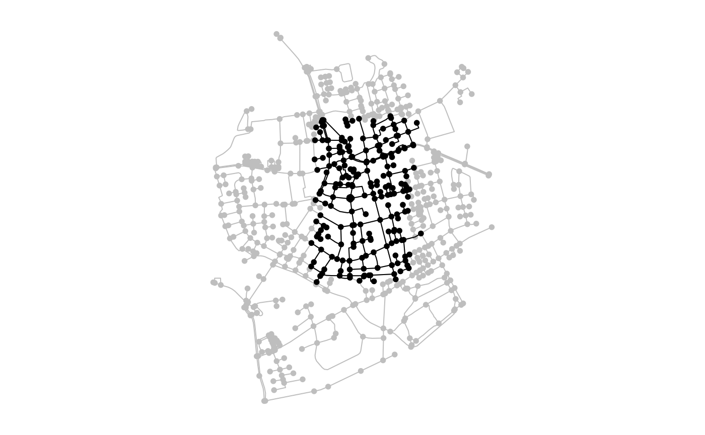
The isolated nodes that remain after filtering the edges can be
easily removed using a combination of a regular
dplyr::filter() verb and the
tidygraph::node_is_isolated() query function.
filtered = net %>%
  activate("edges") %>%
  st_filter(poly, .pred = st_intersects) %>%
  activate("nodes") %>%
  filter(!node_is_isolated())

plot(net, col = "grey")
plot(poly, border = "red", lty = 4, lwd = 4, add = TRUE)
plot(net, col = "grey")
plot(filtered, add = TRUE)
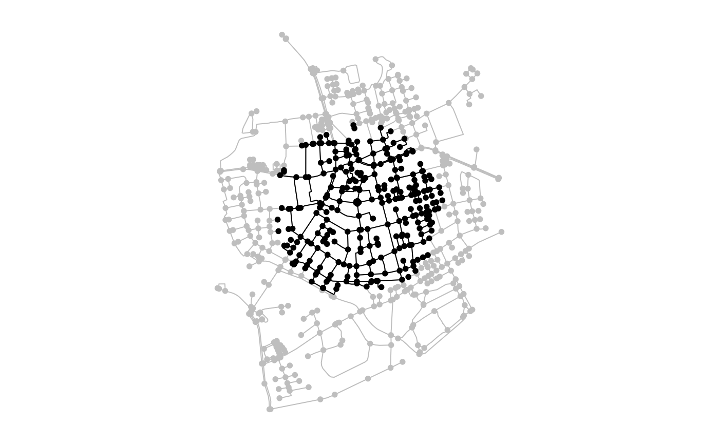
Filtering can also be done with other predicates.
point = st_centroid(st_combine(net))

filtered = net %>%
  activate("nodes") %>%
  st_filter(point, .predicate = st_is_within_distance, dist = 500)

plot(net, col = "grey")
plot(point, col = "red", cex = 3, pch = 20, add = TRUE)
plot(net, col = "grey")
plot(filtered, add = TRUE)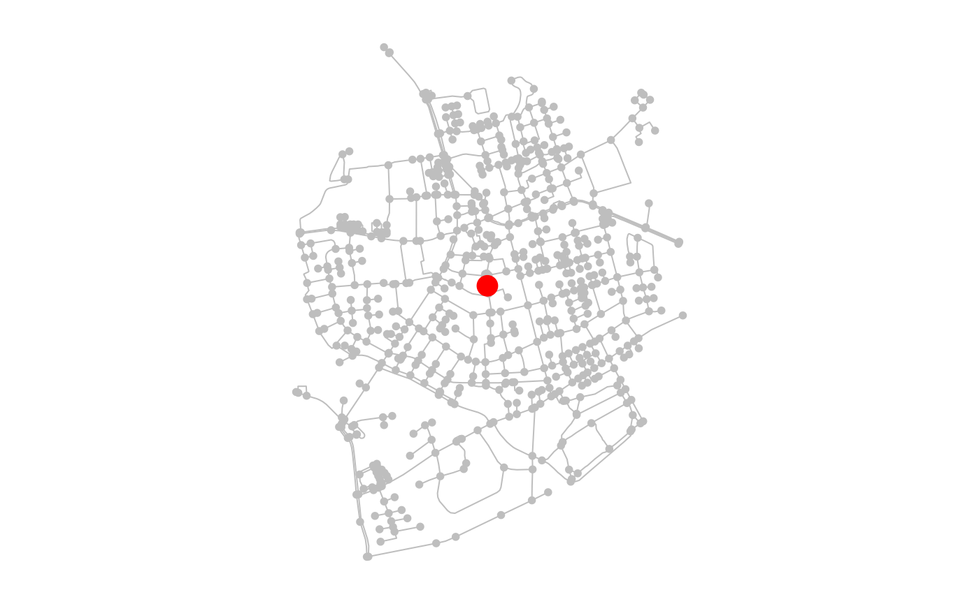
For non-spatial filters applied to attribute columns, simply use
dplyr::filter() instead of
sf::st_filter().
Using spatial node and edge query functions
In tidygraph, filtering information from networks is
done by using specific node or edge query functions inside the
dplyr::filter() verb. An example was already shown above,
where isolated nodes were removed from the network.
In sfnetworks, several spatial predicates are
implemented as node and edge query functions such that you can also do
spatial filtering in tidygraph style. See here
for a list of all implemented spatial node query functions, and here
for the spatial edge query functions.
filtered = net %>%
  activate("edges") %>%
  filter(edge_intersects(poly)) %>%
  activate("nodes") %>%
  filter(!node_is_isolated())

plot(net, col = "grey")
plot(poly, border = "red", lty = 4, lwd = 4, add = TRUE)
plot(net, col = "grey")
plot(filtered, add = TRUE)

A nice application of this in road networks is to find underpassing and overpassing roads (i.e. edges that cross other edges but are not connected at that point). As we can see in the example below, such roads are not present in our Roxel data, which results in a network without edges.
The tidygraph::.E() function used in the example makes
it possible to directly access the complete edges table inside verbs. In
this case, that means that for each edge we evaluate if it crosses with
any other edge in the network. Similarly, we can use
tidygraph::.N() to access the nodes table and
tidygraph::.G() to access the network object as a
whole.
#> # A sfnetwork with 701 nodes and 0 edges
#> #
#> # CRS:  EPSG:3035
#> #
#> # A rooted forest with 701 trees with spatially explicit edges
#> #
#> # Edge data: 0 × 5 (active)
#> # ℹ 5 variables: from <int>, to <int>, name <chr>, type <fct>,
#> #   geometry <LINESTRING [m]>
#> #
#> # Node data: 701 × 1
#>            geometry
#>         <POINT [m]>
#> 1 (4151491 3207923)
#> 2 (4151474 3207946)
#> 3 (4151398 3207777)
#> # ℹ 698 more rows
If you just want to store the information about the investigated
spatial relation, without filtering the network, you can also use the
spatial node and edge query functions inside a
dplyr::mutate() verb.
net %>%
  mutate(in_poly = node_intersects(poly))
#> # A sfnetwork with 701 nodes and 851 edges
#> #
#> # CRS: EPSG:3035
#> #
#> # A directed multigraph with 14 components with spatially explicit edges
#> #
#> # Node data: 701 × 2 (active)
#> geometry in_poly
#> <POINT [m]> <lgl>
#> 1 (4151491 3207923) TRUE
#> 2 (4151474 3207946) TRUE
#> 3 (4151398 3207777) TRUE
#> 4 (4151370 3207673) TRUE
#> 5 (4151408 3207539) TRUE
#> 6 (4151421 3207592) TRUE
#> # ℹ 695 more rows
#> #
#> # Edge data: 851 × 5
#> from to name type geometry
#> <int> <int> <chr> <fct> <LINESTRING [m]>
#> 1 1 2 Havixbecker Strasse residential (4151491 3207923, 4151474 32079…
#> 2 3 4 Pienersallee secondary (4151398 3207777, 4151390 32077…
#> 3 5 6 Schulte-Bernd-Strasse residential (4151408 3207539, 4151417 32075…
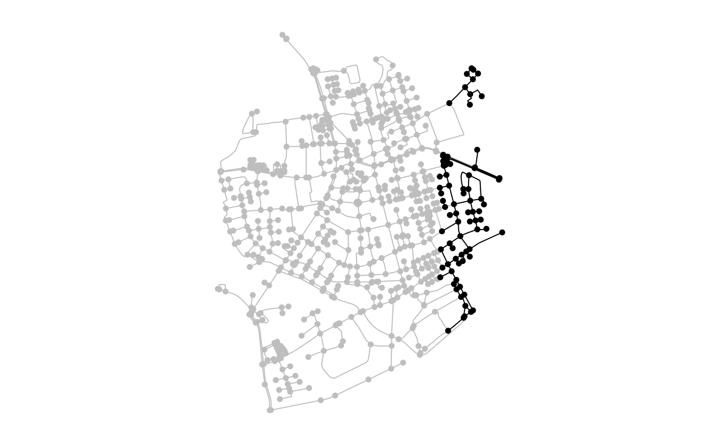
#> # ℹ 848 more rowsBesides predicate query functions, you can also use the coordinate query functions for spatial filters on the nodes. For example:
v = 4152000
l = st_linestring(rbind(c(v, st_bbox(net)["ymin"]), c(v, st_bbox(net)["ymax"])))

filtered_by_coords = net %>%
  activate("nodes") %>%
  filter(node_X() > v)

plot(net, col = "grey")
plot(l, col = "red", lty = 4, lwd = 4, add = TRUE)
plot(net, col = "grey")
plot(filtered_by_coords, add = TRUE)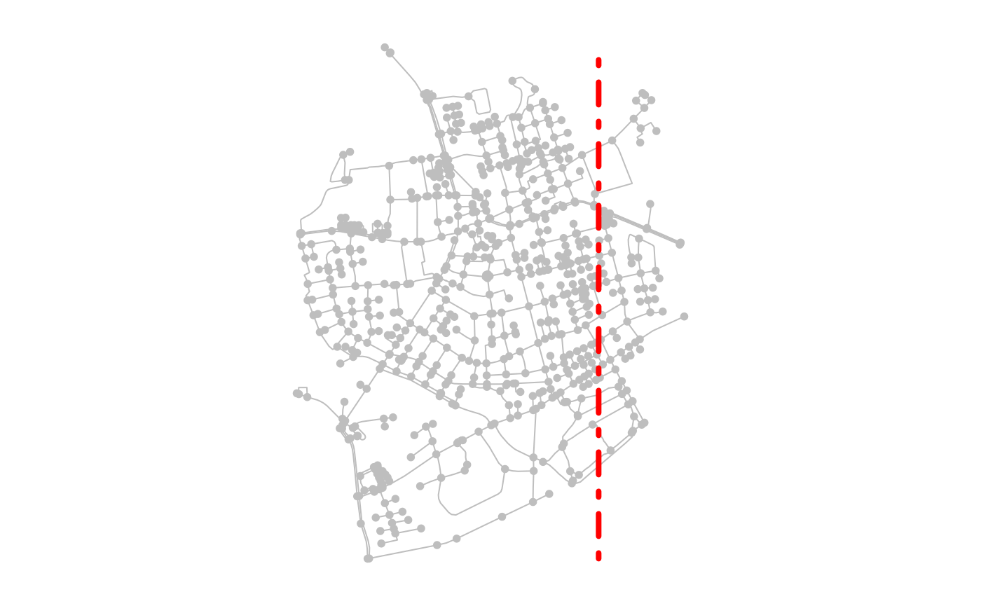
Clipping
Filtering returns a subset of the original geometries, but leaves
those geometries themselves unchanged. This is different from clipping,
in which they get cut at the border of a provided clip feature. There
are three ways in which you can do this:
sf::st_intersection() keeps only those parts of the
original geometries that lie within the clip feature,
sf::st_difference() keeps only those parts of the original
geometries that lie outside the clip feature, and
sf::st_crop() keeps only those parts of the original
geometries that lie within the bounding box of the clip feature.
Note that in the case of the nodes, clipping is not different from
filtering, since point geometries cannot fall party inside and partly
outside another feature. However, in the case of the edges, clipping
will cut the linestring geometries of the edges at the border of the
clip feature (or in the case of cropping, the bounding box of that
feature). To preserve a valid spatial network structure,
sfnetworks adds new nodes at these cut locations.
clipped = net %>%
  activate("edges") %>%
  st_intersection(poly) %>%
  activate("nodes") %>%
  filter(!node_is_isolated())
#> Warning: attribute variables are assumed to be spatially constant throughout
#> all geometries

plot(net, col = "grey")
plot(poly, border = "red", lty = 4, lwd = 4, add = TRUE)
plot(net, col = "grey")
plot(clipped, add = TRUE)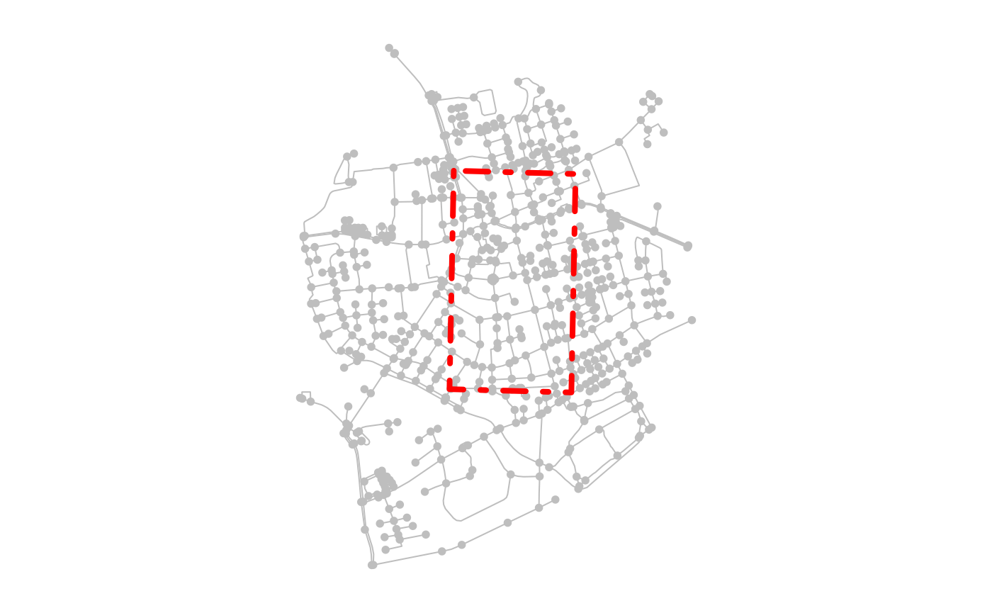
 Note: Neither of the clipping function currently works well with
undirected networks!
Note: Neither of the clipping function currently works well with
undirected networks!
Spatial joins
Using st_join
Information can be spatially joined into a network by using spatial
predicate functions inside the sf function sf::st_join(),
which works as follows: the function is applied to a set of geometries A
with respect to another set of geometries B, and attaches feature
attributes from features in B to features in A based on their spatial
relation. A practical example: when using the predicate
intersects, feature attributes from feature y in B are attached
to feature x in A whenever x intersects with y.
When applying sf::st_join() to a sfnetwork, it is
internally applied to the active element of that network. For example:
joining information into network A with activated nodes, from a set of
polygons B and using the predicate intersects, will attach
attributes from a polygon in B to those nodes that intersect with that
specific polygon. When edges are active, it will attach the same
information but to the intersecting edges instead.
Lets show this with an example in which we first create imaginary postal code areas for the Roxel dataset.
codes = net %>%
  st_make_grid(n = c(2, 2)) %>%
  st_as_sf() %>%
  mutate(post_code = as.character(seq(1000, 1000 + n() * 10 - 10, 10)))

joined = st_join(net, codes, join = st_intersects)
joined
#> # A sfnetwork with 701 nodes and 851 edges
#> #
#> # CRS: EPSG:3035
#> #
#> # A directed multigraph with 14 components with spatially explicit edges
#> #
#> # Node data: 701 × 2 (active)
#> geometry post_code
#> <POINT [m]> <chr>
#> 1 (4151491 3207923) 1020
#> 2 (4151474 3207946) 1020
#> 3 (4151398 3207777) 1020
#> 4 (4151370 3207673) 1020
#> 5 (4151408 3207539) 1020
#> 6 (4151421 3207592) 1020
#> # ℹ 695 more rows
#> #
#> # Edge data: 851 × 5
#> from to name type geometry
#> <int> <int> <chr> <fct> <LINESTRING [m]>
#> 1 1 2 Havixbecker Strasse residential (4151491 3207923, 4151474 32079…
#> 2 3 4 Pienersallee secondary (4151398 3207777, 4151390 32077…
#> 3 5 6 Schulte-Bernd-Strasse residential (4151408 3207539, 4151417 32075…
#> # ℹ 848 more rows
plot(net, col = "grey")
plot(codes, col = NA, border = "red", lty = 4, lwd = 4, add = TRUE)
text(st_coordinates(st_centroid(st_geometry(codes))), codes$post_code, cex = 2)
plot(st_geometry(joined, "edges"))
plot(st_as_sf(joined, "nodes"), pch = 20, add = TRUE)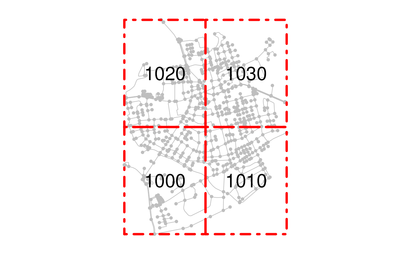
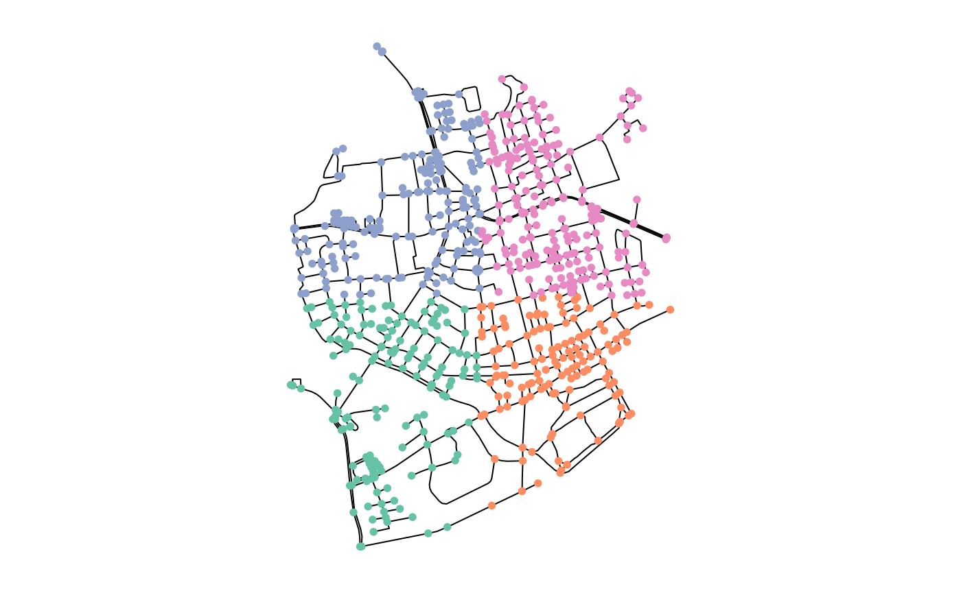
In the example above, the polygons are spatially distinct. Hence,
each node can only intersect with a single polygon. But what would
happen if we do a join with polygons that overlap? The attributes from
which polygon will then be attached to a node that intersects with
multiple polygons at once? In sf this issue is solved by
duplicating such a point as much times as the number of polygons it
intersects with, and attaching attributes of each intersecting polygon
to one of these duplicates. This approach does not fit the network case,
however. An edge can only have a single node at each of its endpoints,
and thus, the duplicated nodes will be isolated and redundant in the
network structure. Therefore, sfnetworks will only join the
information from the first match whenever there are multiple matches for
a single node. A warning is given in that case such that you are aware
of the fact that not all information was joined into the network.
Note that in the case of joining on the edges, multiple matches per edge are not a problem for the network structure. It will simply duplicate the edge (i.e. creating a set of parallel edges) whenever this occurs.
two_equal_polys = st_as_sf(c(poly, poly)) %>%
  mutate(foo = c("a", "b"))

# Join on nodes gives a warning that only the first match per node is joined.
# The number of nodes in the resulting network remains the same.
st_join(net, two_equal_polys, join = st_intersects)
#> Warning: Multiple matches were detected from some nodes. Only the first match
#> is considered
#> # A sfnetwork with 701 nodes and 851 edges
#> #
#> # CRS: EPSG:3035
#> #
#> # A directed multigraph with 14 components with spatially explicit edges
#> #
#> # Node data: 701 × 2 (active)
#> geometry foo
#> <POINT [m]> <chr>
#> 1 (4151491 3207923) a
#> 2 (4151474 3207946) a
#> 3 (4151398 3207777) a
#> 4 (4151370 3207673) a
#> 5 (4151408 3207539) a
#> 6 (4151421 3207592) a
#> # ℹ 695 more rows
#> #
#> # Edge data: 851 × 5
#> from to name type geometry
#> <int> <int> <chr> <fct> <LINESTRING [m]>
#> 1 1 2 Havixbecker Strasse residential (4151491 3207923, 4151474 32079…
#> 2 3 4 Pienersallee secondary (4151398 3207777, 4151390 32077…
#> 3 5 6 Schulte-Bernd-Strasse residential (4151408 3207539, 4151417 32075…
#> # ℹ 848 more rows
# Join on edges duplicates edges that have multiple matches.
# The number of edges in the resulting network is higher than in the original.
net %>%
  activate("edges") %>%
  st_join(two_equal_polys, join = st_intersects)
#> # A sfnetwork with 701 nodes and 1097 edges
#> #
#> # CRS: EPSG:3035
#> #
#> # A directed multigraph with 14 components with spatially explicit edges
#> #
#> # Edge data: 1,097 × 6 (active)
#> from to name type geometry foo
#> <int> <int> <chr> <fct> <LINESTRING [m]> <chr>
#> 1 1 2 Havixbecker Strasse residential (4151491 3207923, 4151474… a
#> 2 1 2 Havixbecker Strasse residential (4151491 3207923, 4151474… b
#> 3 3 4 Pienersallee secondary (4151398 3207777, 4151390… a
#> 4 3 4 Pienersallee secondary (4151398 3207777, 4151390… b
#> 5 5 6 Schulte-Bernd-Strasse residential (4151408 3207539, 4151417… a
#> 6 5 6 Schulte-Bernd-Strasse residential (4151408 3207539, 4151417… b
#> # ℹ 1,091 more rows
#> #
#> # Node data: 701 × 1
#> geometry
#> <POINT [m]>
#> 1 (4151491 3207923)
#> 2 (4151474 3207946)
#> 3 (4151398 3207777)
#> # ℹ 698 more rowsFor non-spatial joins based on attribute columns, simply use a join
function from dplyr (e.g. dplyr::left_join()
or dplyr::inner_join()) instead of
sf::st_join().
Snapping points to their nearest node before joining
Another network specific use-case of spatial joins would be to join
information from external points of interest (POIs) into the nodes of
the network. However, to do so, such points need to have
exactly equal coordinates to one of the nodes. Often this will
not be the case. To solve such situations, you will first need to update
the coordinates of the POIs to match those of their nearest
node. This process is also called snapping. To find the
nearest node in the network for each POI, you can use the sf function
sf::st_nearest_feature().
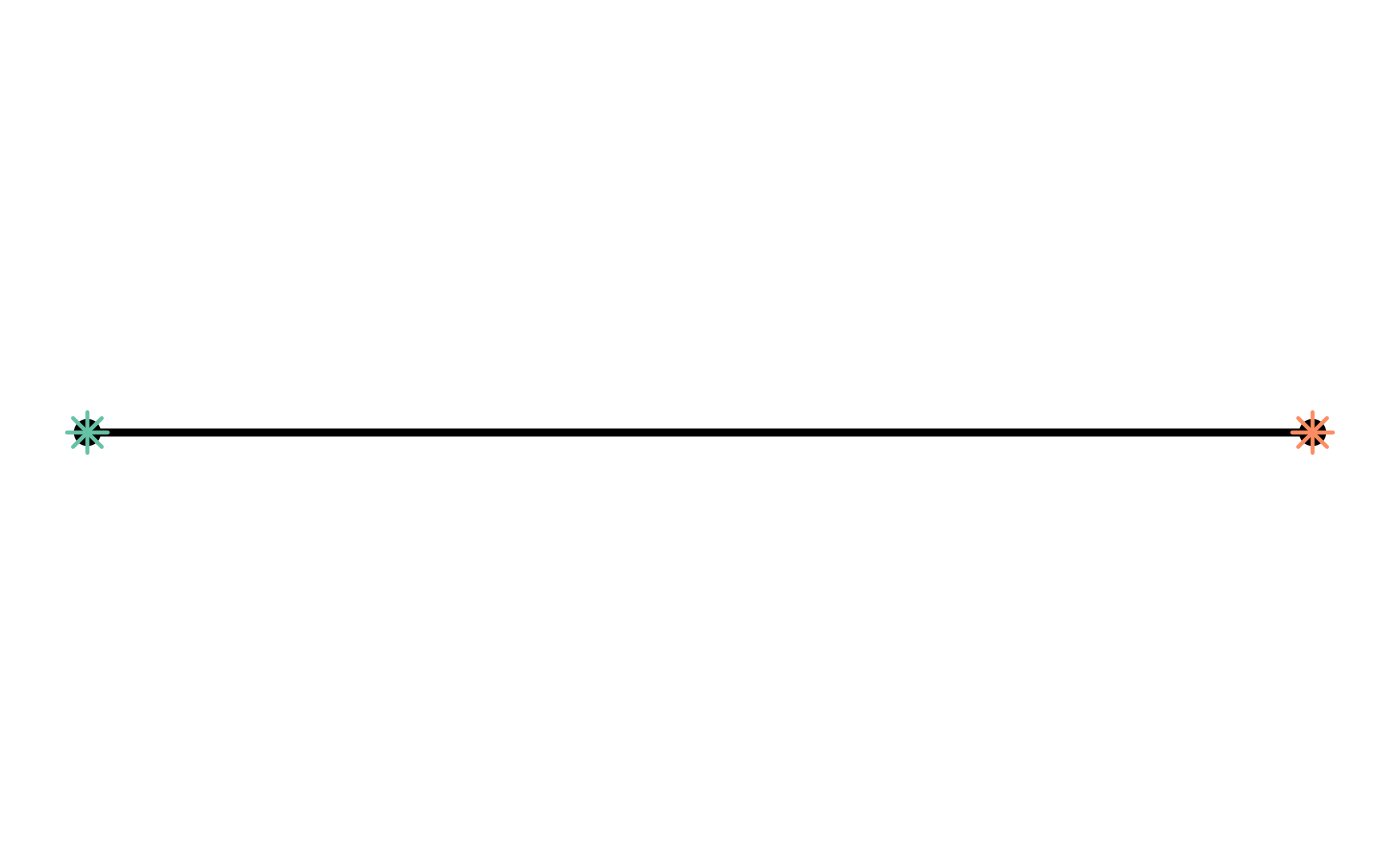
# Create a network.
node1 = st_point(c(0, 0))
node2 = st_point(c(1, 0))
edge = st_sfc(st_linestring(c(node1, node2)))

net = as_sfnetwork(edge)

# Create a set of POIs.
pois = data.frame(poi_type = c("bakery", "butcher"),
                  x = c(0, 0.6), y = c(0.2, 0.2)) %>%
  st_as_sf(coords = c("x", "y"))

# Find indices of nearest nodes.
nearest_nodes = st_nearest_feature(pois, net)

# Snap geometries of POIs to the network.
snapped_pois = pois %>%
  st_set_geometry(st_geometry(net)[nearest_nodes])

# Plot.
plot_connections = function(pois) {
  for (i in seq_len(nrow(pois))) {
    connection = st_nearest_points(pois[i, ], net)[nearest_nodes[i]]
    plot(connection, col = "grey", lty = 2, lwd = 2, add = TRUE)
  }
}

plot(net, cex = 2, lwd = 4)
plot_connections(pois)
plot(pois, pch = 8, cex = 2, lwd = 2, add = TRUE)
plot(net, cex = 2, lwd = 4)
plot(snapped_pois, pch = 8, cex = 2, lwd = 2, add = TRUE)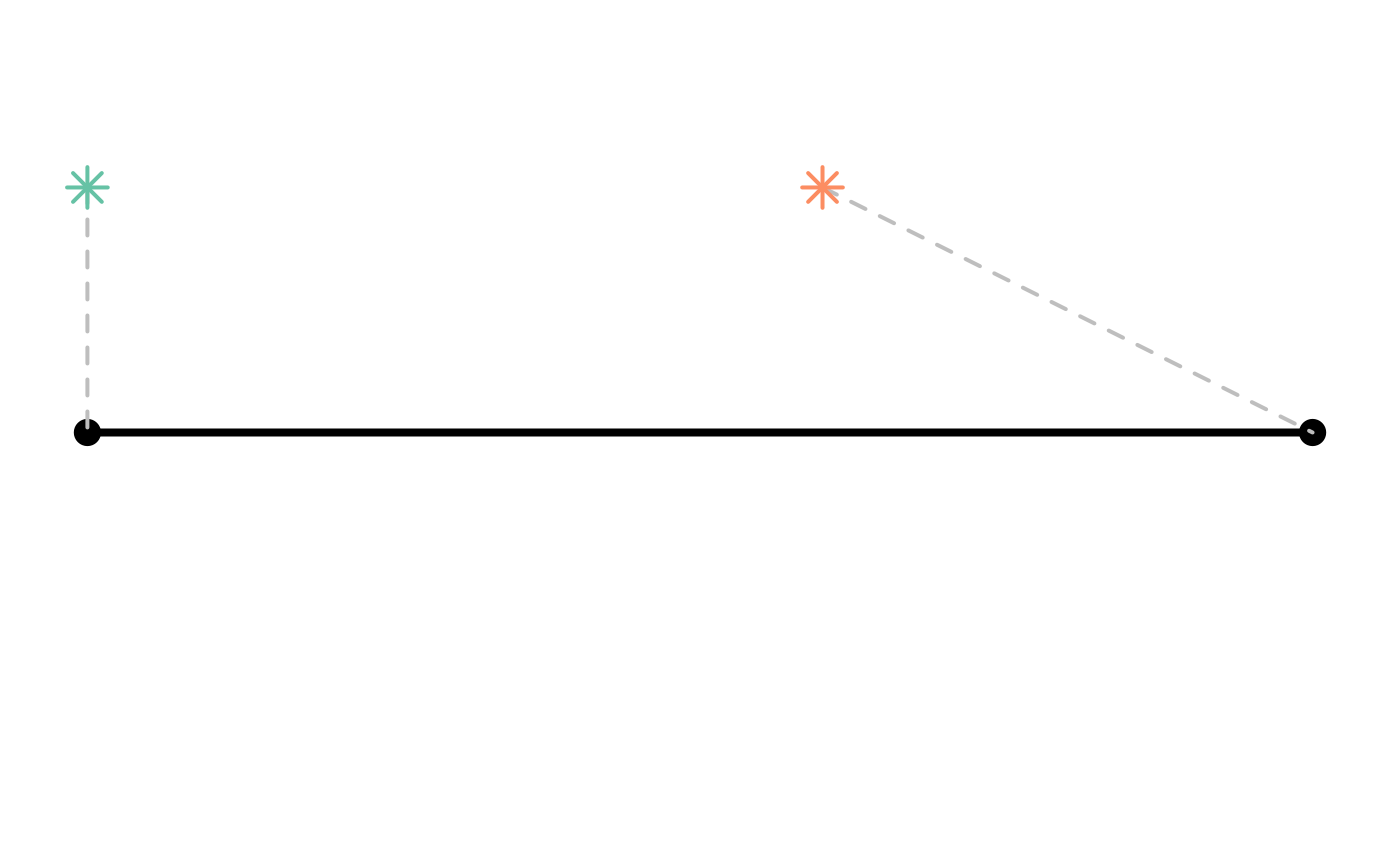
After snapping the POIs, we can use sf::st_join() as
expected. Do remember that if multiple POIs are snapped to the same
node, only the information of the first one is joined into the
network.
st_join(net, snapped_pois)#> # A sfnetwork with 2 nodes and 1 edges
#> #
#> # CRS: NA
#> #
#> # A rooted tree with spatially explicit edges
#> #
#> # Node data: 2 × 2 (active)
#> x poi_type
#> <POINT> <chr>
#> 1 (0 0) bakery
#> 2 (1 0) butcher
#> #
#> # Edge data: 1 × 3
#> from to x
#> <int> <int> <LINESTRING>
#> 1 1 2 (0 0, 1 0)Blending points into a network
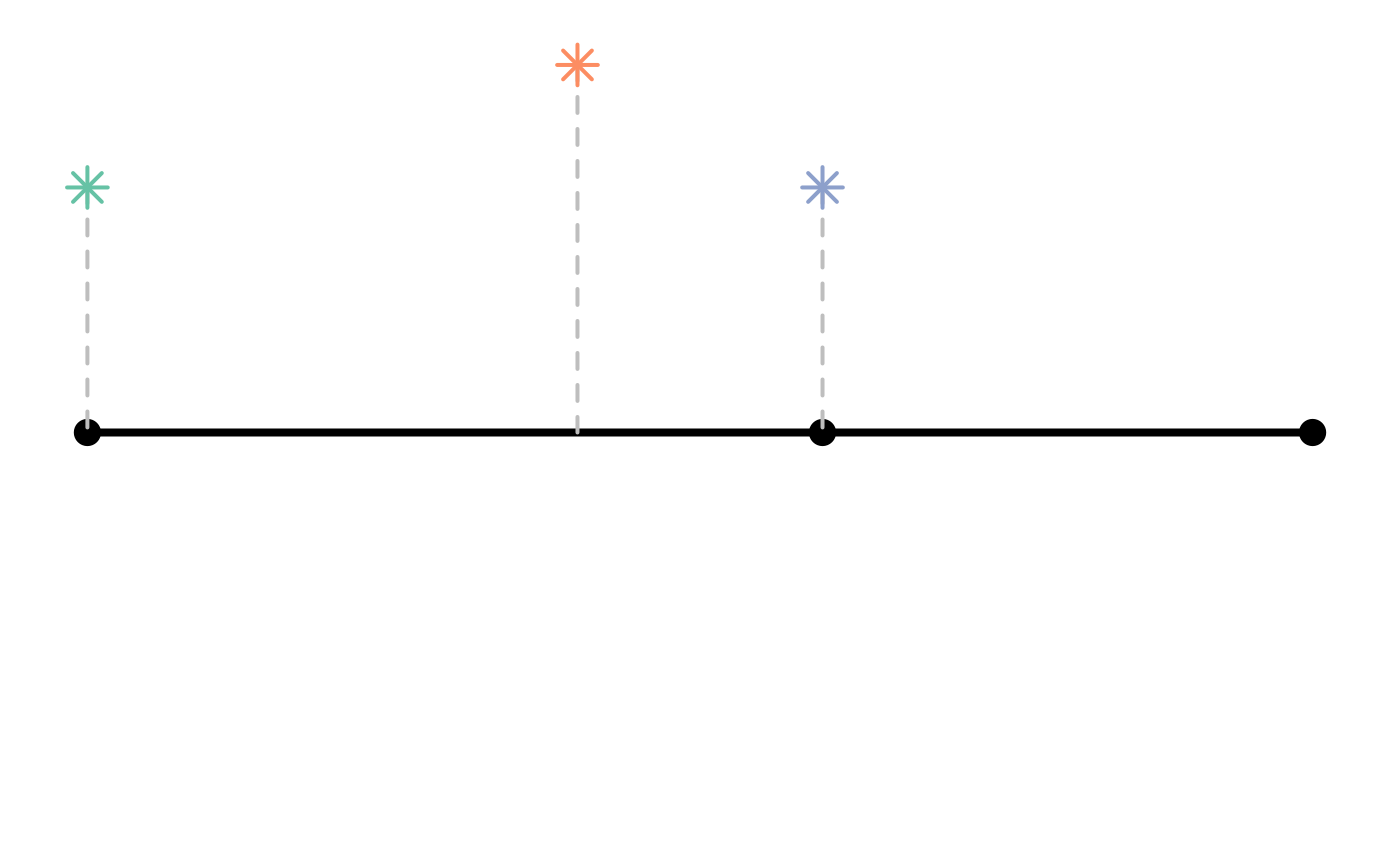
In the example above, it makes sense to include the information from the first POI in an already existing node. For the second POI, however, its nearest node is quite far away relative to the nearest location on its nearest edge. In that case, you might want to split the edge at that location, and add a new node to the network. For this combination process we use the metaphor of throwing the network and POIs together in a blender, and mix them smoothly together.
The function st_network_blend() does exactly that. For
each POI, it finds the nearest location
on the nearest edge
.
If
is an already existing node
(i.e.
is an endpoint of
),
it joins the information from the POI into that node. If
is not an already existing node, it subdivides
at
,
adds
as a new node to the network, and joins the information from
the POI into that new node. For this process, it does not
matter if
is an interior point in the linestring geometry of
.
blended = st_network_blend(net, pois)
blended
#> # A sfnetwork with 3 nodes and 2 edges
#> #
#> # CRS: NA
#> #
#> # A rooted tree with spatially explicit edges
#> #
#> # Node data: 3 × 2 (active)
#> poi_type x
#> <chr> <POINT>
#> 1 bakery (0 0)
#> 2 NA (1 0)
#> 3 butcher (0.6 0)
#> #
#> # Edge data: 2 × 3
#> from to x
#> <int> <int> <LINESTRING>
#> 1 1 3 (0 0, 0.6 0)
#> 2 3 2 (0.6 0, 1 0)
plot_connections = function(pois) {
  for (i in seq_len(nrow(pois))) {
    connection = st_nearest_points(pois[i, ], activate(net, "edges"))
    plot(connection, col = "grey", lty = 2, lwd = 2, add = TRUE)
  }
}

plot(net, cex = 2, lwd = 4)
plot_connections(pois)
plot(pois, pch = 8, cex = 2, lwd = 2, add = TRUE)
plot(blended, cex = 2, lwd = 4)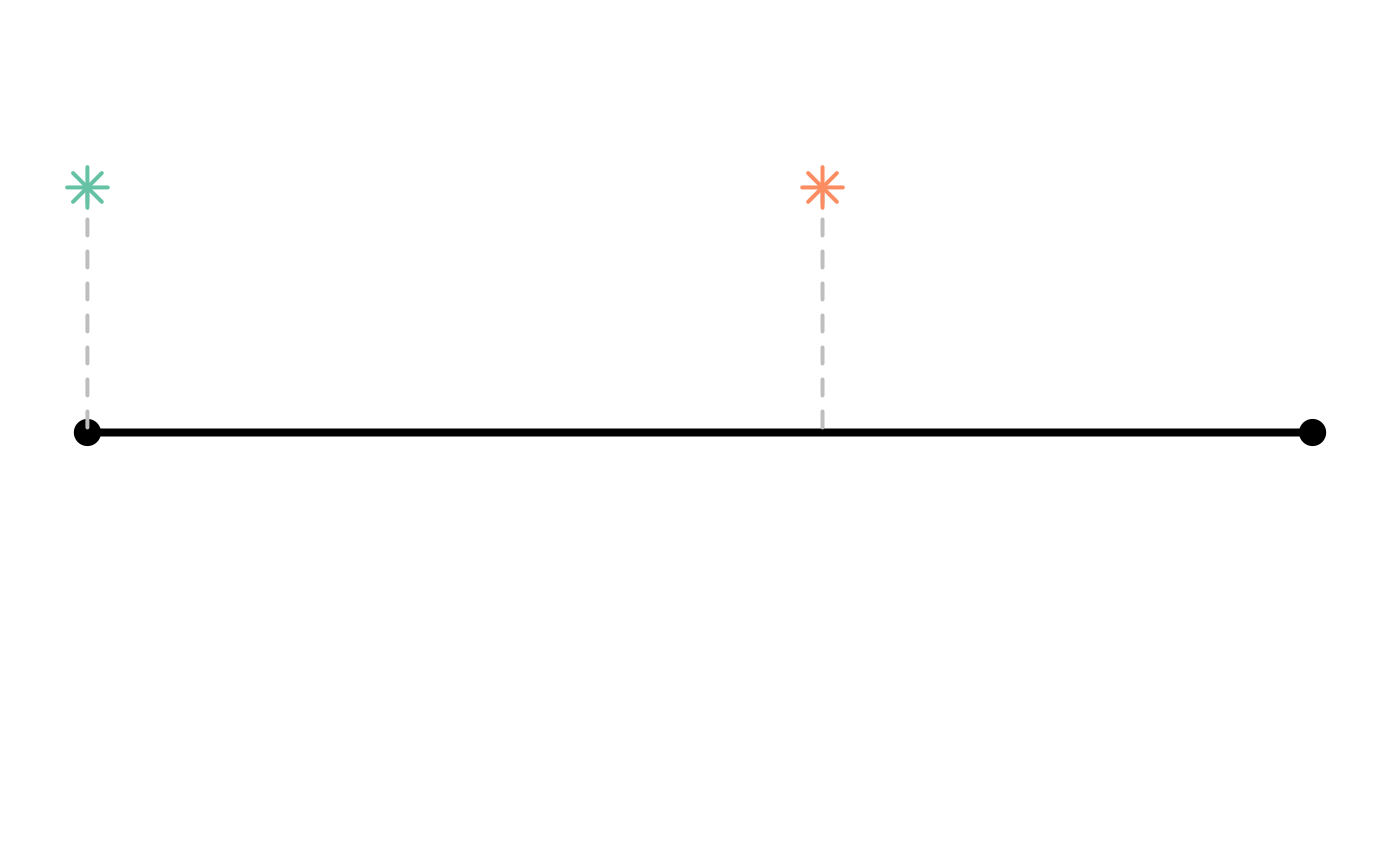

The st_network_blend() function has a
tolerance parameter, which defines the maximum distance a
POI can be from the network in order to be blended in. Hence, only the
POIs that are at least as close to the network as the tolerance distance
will be blended, and all others will be ignored. The tolerance can be
specified as a non-negative number. By default it is assumed its units
are meters, but this behaviour can be changed by manually setting its
units with units::units().
pois = data.frame(poi_type = c("bakery", "butcher", "bar"),
                  x = c(0, 0.6, 0.4), y = c(0.2, 0.2, 0.3)) %>%
  st_as_sf(coords = c("x", "y"))

blended = st_network_blend(net, pois)
blended_with_tolerance = st_network_blend(net, pois, tolerance = 0.2)

plot(blended, cex = 2, lwd = 4)
plot_connections(pois)
plot(pois, pch = 8, cex = 2, lwd = 2, add = TRUE)
plot(blended_with_tolerance, cex = 2, lwd = 4)
plot_connections(pois)
plot(pois, pch = 8, cex = 2, lwd = 2, add = TRUE)
There are a few important details to be aware of when using
st_network_blend(). Firstly: when multiple POIs have the
same nearest location on the nearest edge, only the first of
them is blended into the network. This is for the same reasons as
explained before: in the network structure there is no clear approach
for dealing with duplicated nodes. By arranging your table of POIs with
dplyr::arrange() before blending you can influence which
(type of) POI is given priority in such cases.
Secondly: when a single POI has multiple nearest edges, it is only
blended into the first of these edges. Therefore, it might be a good
idea to run the to_spatial_subdivision() morpher after
blending, such that intersecting but unconnected edges get connected.
See the Network
pre-processing and cleaning vignette for more details.
Lastly: it is important to be aware of floating point precision. See the discussion in this GitHub issue for more background. In short: due to internal rounding of rational numbers in R it is actually possible that even the intersection point between two lines is not evaluated as intersecting those lines themselves. Sounds confusing? It is! But see the example below:
# Create two intersecting lines.
p1 = st_point(c(0.53236, 1.95377))
p2 = st_point(c(0.53209, 1.95328))
l1 = st_sfc(st_linestring(c(p1, p2)))

p3 = st_point(c(0.53209, 1.95345))
p4 = st_point(c(0.53245, 1.95345))
l2 = st_sfc(st_linestring(c(p3, p4)))

# The two lines share an intersection point.
st_intersection(l1, l2)
#> Geometry set for 1 feature
#> Geometry type: POINT
#> Dimension:     XY
#> Bounding box:  xmin: 0.5321837 ymin: 1.95345 xmax: 0.5321837 ymax: 1.95345
#> CRS:           NA
#> POINT (0.5321837 1.95345)

# But this intersection point does not intersects the line itself!
st_intersects(l1, st_intersection(l1, l2), sparse = FALSE)
#>       [,1]
#> [1,] FALSE

# The intersection point is instead located a tiny bit next to the line.
st_distance(l1, st_intersection(l1, l2))
#>              [,1]
#> [1,] 4.310191e-17
That is: you would expect an intersection with an edge to be blended
into the network even if you set tolerance = 0, but in fact
that will not always happen. To avoid having these problems, you can
better set the tolerance to a very small number instead of zero.
net = as_sfnetwork(l1)
p = st_intersection(l1, l2)

plot(l1)
plot(l2, col = "grey", lwd = 2, add = TRUE)
plot(st_network_blend(net, p, tolerance = 0), lwd = 2, cex = 2, add = TRUE)
#> Warning: No points were blended. Increase the tolerance distance?
plot(l1)
plot(l2, col = "grey", lwd = 2, add = TRUE)
plot(st_network_blend(net, p, tolerance = 1e-10), lwd = 2, cex = 2, add = TRUE)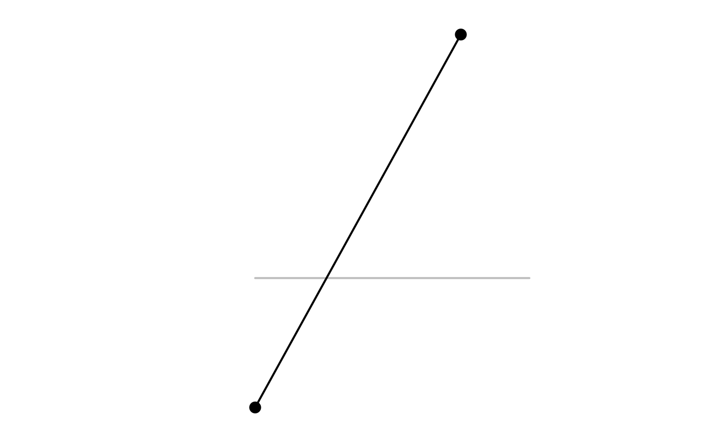

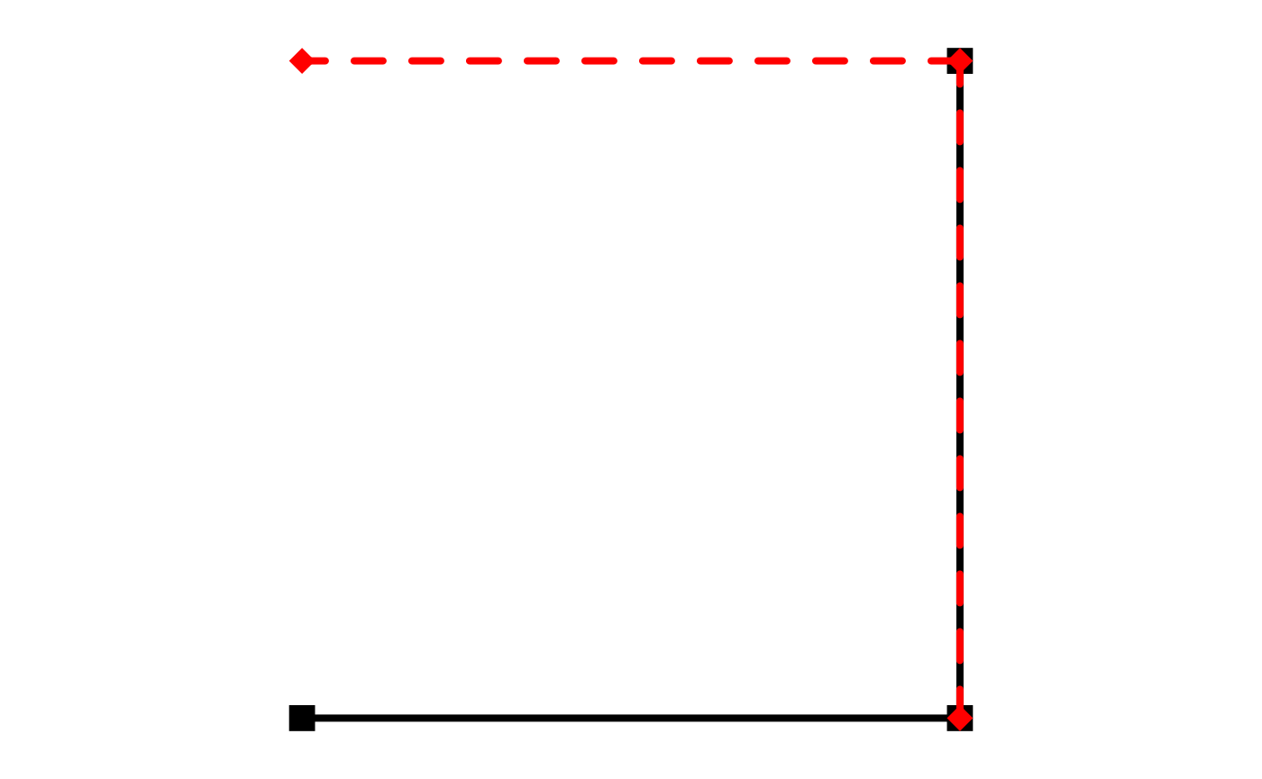
Joining two networks
In the examples above it was all about joining information from
external features into a network. But how about joining two networks?
This is what the st_network_join() function is for. It
takes two sfnetworks as input and makes a spatial full join on the
geometries of the nodes data, based on the equals spatial
predicate. That means, all nodes from network x and all nodes
from network y are present in the joined network, but if there were
nodes in x with equal geometries to nodes in y, these nodes become a
single node in the joined network. Edge data are combined using
a dplyr::bind_rows() semantic, meaning that data are
matched by column name and values are filled with NA if
missing in either of the networks. The from and to
columns in the edge data are updated automatically such that they
correctly match the new node indices of the joined network. There is no
spatial join performed on the edges. Hence, if there is an edge in x
with an equal geometry to an edge in y, they remain separate edges in
the joined network.
node3 = st_point(c(1, 1))
node4 = st_point(c(0, 1))
edge2 = st_sfc(st_linestring(c(node2, node3)))
edge3 = st_sfc(st_linestring(c(node3, node4)))

net = as_sfnetwork(c(edge, edge2))
other_net = as_sfnetwork(c(edge2, edge3))

joined = st_network_join(net, other_net)
joined
#> # A sfnetwork with 4 nodes and 4 edges
#> #
#> # CRS: NA
#> #
#> # A directed acyclic multigraph with 1 component with spatially explicit edges
#> #
#> # Node data: 4 × 1 (active)
#> x
#> <POINT>
#> 1 (0 0)
#> 2 (1 0)
#> 3 (1 1)
#> 4 (0 1)
#> #
#> # Edge data: 4 × 3
#> from to x
#> <int> <int> <LINESTRING>
#> 1 1 2 (0 0, 1 0)
#> 2 2 3 (1 0, 1 1)
#> 3 2 3 (1 0, 1 1)
#> # ℹ 1 more row
plot(net, pch = 15, cex = 2, lwd = 4)
plot(other_net, col = "red", pch = 18, cex = 2, lty = 2, lwd = 4, add = TRUE)
plot(joined, cex = 2, lwd = 4)